Chapter 2 - Discrete-time signals and systems
Discrete-time signals, energy and power of discrete signals, signal symmetries, block diagrams, classification, convolution.
Examples of Discrete time signals
Discrete time signal
$$x(n)=\sin\left(2\pi\frac{1}{8}n\right)\approx\\\{\dots~-1~-0.7~\underline{0}~0.7~1~0.7~\dots\}$$
The underline indicates `n=0`.
Discrete time systems
Average of three last values of `x(n)`:
$$y(n)=\frac{1}{3}x(n)+\frac{1}{3}x(n-1)+\frac{1}{3}x(n-2)$$
A stable system decaying at a rate of 0.9:
$$y(n)=0.9y(n-1)+x(n)$$
A unstable system diverging at a rate of 1.1:
$$y(n)=1.1y(n-1)+x(n)$$
Discrete time signals
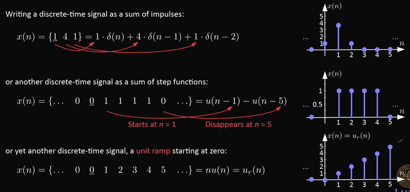
The Dirac delta function is used for impulses.
$$\delta(n)=\begin{cases}1&\text{if }n=0\\0&\text{otherwise}\end{cases}$$
The Step function (Heaviside/unit).
$$u(n)=\begin{cases}1&\text{if }n\geq0\\0&\text{otherwise}\end{cases}$$
These two functions can be combined to make other signals.
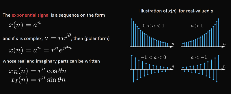
Exponential signals
Energy and Power of discrete signals
The energy of a signal is defined as:
$$E\equiv\sum_{n=-\infty}^{\infty}|x(n)|^2$$
The average power of a signal is defined as:
$$P\equiv\lim\limits_{N\to\infty}\frac{1}{2N+1}\sum\limits_{n=-N}^{N}|x(n)|^2$$
Even if a signal has infinite energy, the average power could still be finite.
We can also express the energy as:
$$E\equiv\lim\limits_{N\to\infty}E_N$$
where
$$E_N\equiv\sum_{n=-N}^N|x(n)|^2$$
Energy Signal and Power Signal
$$\text{energy signal}\iff 0 < E < \infty,P=0$$
$$\text{power signal}\iff 0 < P < \infty,E=\infty$$
Signal symmetries
A signal is symmetric or even if `x(n) = x(-n)`.
A signal is antisymmetric or odd if `x(n) = -x(-n)`.
Any signal `x(n)` can be written as a sum of an odd and even signal.
$$
\begin{split}
x(n) &= x_e(n) + x_o(n) \\
x_e(n) &= \frac{1}{2}(x(n)+x(-n)) \\
x_o(n) &= \frac{1}{2}(x(n) - x(-n))
\end{split}
$$
Block diagrams
For block diagrams see lecture slides or chapter 2.2.2 in the book.
Classification
We call systems different things depending on their properties, a system is called:
- static: if without memory
- dynamic: if without memory,
- time-invariant: where I/O characteristics don't change with time,
- time-variant: where I/O characteristics change with time,
- linear system: when it satisfies the superposition principle,
- non-linear system: when it doesn't satisfy the superposition principle,
- causal: where the output at any time only depends on the current and past inputs,
- bounded-input bounded-output (BIBO) stable: where bounded inputs `|x(n)| \leq M_x` always produce bounded outputs `|y(n)| \leq M_y`.
LTI systems
Focus is on Linear Time-Invariant (LTI) systems in this course.
$$\delta(n) \rightarrow \boxed{\text{LTI system}} \rightarrow h(n)$$
The impulse response `h(n)` of an LTI system is the output signal when the input signal is a unit impulse `\delta(n)` at time `n=0`.
Discrete time convolution
An arbitrary signal can be written as the sum of delayed impulses:
$$x(n) = \sum_{k=-\infty}^\infty x(k)\delta(n-k)$$
Since LTI systems are linear and time-invariant the output `y(n)` will be the sum of impulse responses:
$$y(n) = x(n)*h(n) = \sum_{k=-\infty}^\infty x(k)h(n-k)$$
Convolution properties
Unit impulse is the identity element of convolution:
$$x(n)*\delta(n) = \sum_{k=-\infty}^\infty x(k)\delta(n-k) = x(n)$$
Convolution fulfills the:
- commutative law: \(x*h = h*x\),
- associative law: \((x*h_1)*h_2 = x * (h_1*h_2)\),
- distributive law: \(x*(h_1+h_2) = x*h_1 + x*h_2\)
Convolution length
If we have two finite-length signals `x(n)` and `h(n)` with lengths `M` and `N` then the convolution \(y(n) = x(n) * h(n)\) will have length `M+N-1`
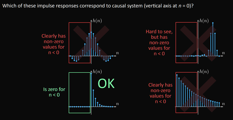
Causality
An LTI system is only causal if its impulse response fulfills: `h(n) = 0` for all `n < 0`.
Constant-coefficient difference equations
If we take the example of a recursive system:
$$y(n) = ay(n-1)+x(n)$$
We can rewrite it in terms of the memory from `n=0`:
$$y(n) = a^{n+1}y(-1) + \sum_{k=0}^n a^kx(n-k)$$
Constant-coefficient difference equations describe LTI systems.
Zero-state response
If the state of the system at `n=0` is zero (relaxed): e.g. `y(-1)=0` we get the zero-state response:
$$y_{zs}(n) = \sum_{k=0}^na^kx(n-k)$$
Zero-input response
If the input signal is zero, `x(n) = 0`, we get the zero-input response (natural response):
$$y_{zi}(n) = a^{n+1}y(-1)$$
The output signal is the sum: `y(n) = y_{zi}(n) + y_{zs}(n)`.